Introduction
When I started in electronics as a profession, way back in 1998, as an apprentice electronics technician, there were a series of treasured design documents that the boss kept in a special green and well-worn manila folder, safe under lock and key in his filing cabinet. Amongst these documents were the active filter coefficient tables, copies of which I am providing here.Back in 1998 the internet was not the huge repository of information that it is today, and documents like these were felt to be worth their weight in gold. However, even today, I still find the tables presented here useful, so Ive decided to put them onto the World Wide Web. I do not know the provenance of these coefficient tables, other than that they were obviously computed by someone with a bit of a mathematical bent and that they were already of some vintage in 1998, as, judging by the quality of the photocopies that my old boss posessed, they were numerous generations removed from the originals.
Requiring only some rather basic arithmetic, detailed here, the tables permit the design of both low-pass and high-pass active filters of any number of poles between two and ten. Coefficient values are given for Bessel, Butterworth and Chebyshev filter responses. There are six separate sets of Chebyshev response coefficients, to design filters with an amplitude ripple in the passband of either 0.1 dB, 0.25 dB, 0.5 dB, 1 dB, 2 dB or 3 dB; the greater the ripple, the sharper, or more abrupt, the amplitude attenuation beyond the cut-off frequency.
For filter responses of more than three poles, the filters are constructed from a combination of individual filter stages of either two or three poles each. For example, a 10-pole filter is realised by a cascade of five 2-pole stages while a 5-pole filter is realised by a 3-pole stage followed by a 2-pole stage. The former requires five individual op-amps and the latter requires two. A noteworthy aspect of these tables is that the coefficient values were figured out for making a 3-pole stage with a single op-amp, which is rarely seen. This has the potential benefit of economising on the number of actual op-amps required. Multiple-pole active filters comprised of individual sections of greater than two poles are seldom seen in the literature as the coefficient values are much harder to figure out.
A design example
Although the tables provide capacitor value coefficients normalized to Farads ostensibly for a low-pass filter configuration, once the low-pass filter is computed it can be transformed into a high-pass design simply by swapping the capacitors for resistors and the resistors for capacitors and computing the substitute component values from the respective reactances. A worked example is given.Resistances are initially normalised to one ohm, the frequency of operation to 1 / (2*pi) Hz and each stage is a unity-gain, voltage-controlled-voltage-source (VCVS) filter, based on a single op-amp wired as a voltage-follower.
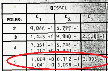
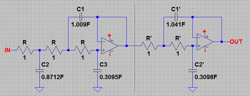
As a design example, a 5-pole low-pass Bessel filter with a cut-off frequency of 1 kHz will be computed. It will then be transformed into a high-pass filter. The filter is comprised of a 3-pole VCVS filter stage followed by a 2-pole VCVS filter stage. The 5-pole Bessel coefficient values from the table are transferred to the filter schematic as follows:
C1 = 160.59 uF
C2 = 138.66 uF
C3 = 49.26 uF
C1' = 165.68 uF
C2' = 49.31 uF
As the these aren't particularly desirable values, the next step is to scale the largest value of each stage to a practical value of capacitance. If 10 nF is chosen for both C1 and C1, scaling factors m and m are computed thus:
m = 160.59 uF / 10 nF = 16059
m = 165.68 uF / 10 nF = 16568
The values of the remaining capacitors of each stage are computed by dividing by the respective scaling factors:
C2 = 138.66 uF / m = 8.63 nF
C3 = 49.31 uF / m = 3.07 nF
C2 = 49.31 uF / m = 2.98 nF
The last step is to scale the resistors by multiplying by the respective scaling factors used to divide down the value of the capacitors:
R = R * m = 16059 ohms
R = R * m = 16568 ohms
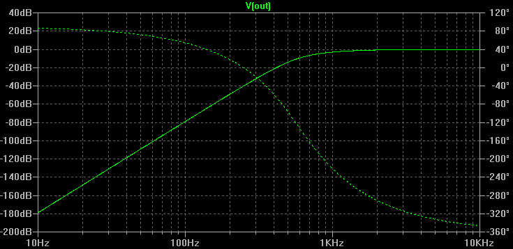
R is close enough to 16 k. R can be made from a 16 k resistor in series with a 560 ohm resistor. C3 and C2 are close enough to 3 nF to be each made up of two 1.5 nF capacitors in parallel. The value for C2 can be arrived at by connecting a 3.9 nF capacitor in parallel with a 4.7 nF capacitor. Here is the simulated amplitude and phase response of the filter with these component values:
Low-pass to high-pass transformation
The first step is to substitute all of the capacitors for resistors and all of the resistors for capacitors: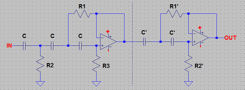
Xc = 1 / (2*pi*f*C)
Rearranging to solve for C:
C = 1 / (2*pi*f*Xc)
To compute the capacitor values of the filter, Xc is taken as the value, in ohms, of the resistors previously occupying the positions:
C = 1 / (2*pi*f*16059) = 9.91 nF
C = 1 / (2*pi*f*16568) = 9.61 nF
The resistors, alternatively, are given the values, in ohms, equal to the capacitive reactances of the capacitors previously occupying the positions:
R1 = 1 / (2*pi*f* 10 nF) = 15915 ohms
R2 = 1 / (2*pi*f* 8.63 nF) = 18442 ohms
R3 = 1 / (2*pi*f* 3.07 nF) = 51842 ohms
R1 = 1 / (2*pi*f* 10 nF) = 15915 ohms
R2 = 1 / (2*pi*f* 2.98 nF) = 53408 ohms
Suppose that we wish to scale to more convenient values for the capacitors, to avoid the need for connecting multiple devices in parallel to achieve the desired values. Selecting a standard value of 22 nF for both C and C' yields the scaling factors:
m = 22 nf / 9.91 nF = 2.22
m = 22 nF / 9.61 nF = 2.29
To maintain the same cut-off frequency the resistors must be scaled in the opposite direction by the same factors. The capacitors were scaled up (to 22 nF), so the resistors must be scaled down:
R1 = 15915 / m = 7169 ohms
R2 = 18442 / m = 8307 ohms
R3 = 51842 / m = 23352 ohms
R1 = 15915 / m = 6950 ohms
R2 = 53408 / m = 23322 ohms
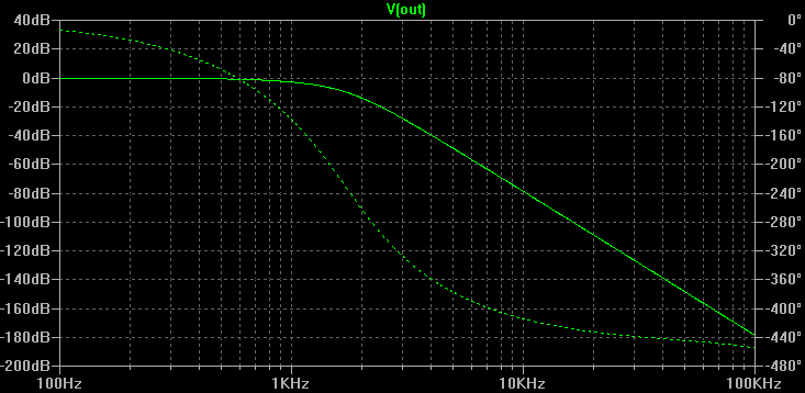
Here is the simulated amplitude and phase response of the high-pass filter with these component values: