A 3-Dimensional Projective Unit

This is a unit that I designed and built to further my experiments in analog computation. By mapping a 3-fold space on a 2-dimensional screen, it generates 3-dimensional perspective displays on an X-Y oscilloscope CRT for any object or system (reproduced by either a generator circuit or an electrical analog) which is defined in three dimensions by x, y and z Cartesian co-ordinates:

A full 0-to-360 degrees of user-variable rotation of the projection is available, independently, on both the x and y axes. The angles of rotation for both these axes are adjustable (in step resolutions of 1 degree) by means of two pairs of ADC-read “coarse” and “fine” potentiometer knobs provided on the front panel of the unit, while the angle of rotation for each axis is displayed digitally, on two sets of three 7-segment LED displays.

The circuitry of the unit presented here is an elaboration and expansion upon, using modern components and techniques, the basic 3-dimensional scheme described in chapter 9 of Ref. [1] (from hereon referred to as Mackay & Fisher), the relevant pages of which can be downloaded here. I do understand that I am technically in violation of copyright by providing these 4 pages in total for viewing and distribution, but the text is a rather old one (1962) and has been out print for several decades as it concerns a wholly obsolete technology. I'm quite sure nobody will mind.

For my implementation I functionally reproduced the transformation units described by Mackay & Fisher to the extent necessary to generate, from the x, y and z input signals, the signals:

x’ = x cos θ – z sin θ
y’ = y sin Φ – z’ cos Φ
z’ = x sin θ + z cos θ

Where:

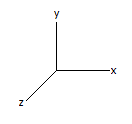
θ is the angle of rotation about the y axis and
Φ is the angle of rotation about the x axis.

x' and y' are the horizontal and vertical deflection signals for the oscilloscope display respectively and z' is simply required to compute y'.

Instead of using a pair of the novel (but no longer available) quad-wiper, sine-cosine law potentiometers as detailed by Mackay & Fisher, I used software-ganged 8-bit digital potentiometers controlled by a microcontroller (uC) programmed with a sine-cosine look-up table. The only change I made to the fundamental operation of the system of Mackay & Fisher was to follow each potentiometer wiper with a switchable inverting amplifier, controlled by the uC. This addition, in a manner to be explained, permitted me to expand the adjustable range for the x-axis and the y-axis angles of rotation to a full 360 degrees each. The design by Mackay & Fisher was limited to a 0-to-90 degree range.

The reason the design by Mackay & Fisher was limited to a 90 degree range in the angles of projection was because a potentiometer by itself can only multiply a variable by a constant having a value in the range of 0 to 1. Figure 1 immediately below shows sine and cosine functions representing the multiplication constants. As can be seen, if operation is limited to the range in which both constants are somewhere between the values of of 0 and 1, the angle(s) of rotation cannot extend beyond pi/2 radians; that being equal to 90 degrees.

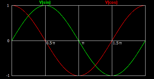
Figure 1

If, however, the multiplication coefficients can be extended in range, from 0 to 1, to -1 to 1, operation is permissible over the full 360 degrees. This is where the switchable inverting stages following the wipers of each digital potentiometer come into play. With reference to the schematic diagram, these six (identical) switchable inverting stages are based on op-amps U4A through U4D, U7B, U7D and JFETs Q1 through Q6.

Consider the switchable inverting stage based on op-amp U4A and JFET Q1. If Q1 is in the OFF state, the non-inverting input of U4A is presented with the (buffered) signal voltage from the wiper of the stages respective multiplication potentiometer. Input resistor R12 is therefore effectively bootstrapped and U4A simply operates as a unity gain, non-inverting buffer; the respective potentiometer retains a range of 0 to 1 for the multiplication constant. If, however, JFET Q1 is in the ON state, the non-inverting input of U4A is effectively grounded and the stage behaves as a unity gain inverting amplifier; the multiplication constant now has a range of 0 to -1.

Coordinated switching of the JFETs, such that the switchable inverting stage for each sine and cosine function operates in the appropriate mode during each 90 degree quadrant is performed by firmware in the uC (see subroutine sincostable() of the C program listing)

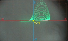
Immediately below are some oscilloscope screen photos of the Rössler attractor, in both 2-D plane views and 3-D projective views. For these displays my Rössler attractor circuit was used as the x-y-z signal source for the projection unit. For each photo the user settings of the x and y angles of rotation are given.

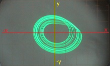
Top-down, 2-D plane view (X-rotation = 90, Y-rotation = 0)

Edge-on, 2-D plane view (X-rotation = 180, Y-rotation = 0)

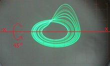
Edge-on, 2-D plane view, 45 degrees of rotation on y-axis (X-rotation = 180, Y-rotation = 45)

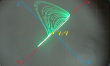
3-D projective view, 45 degrees of rotation on x-axis (X-rotation = 135, Y-rotation = 0)

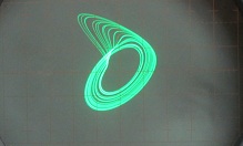
3-D projective view, 45 degrees of rotation on both x and y axes (X-rotation = 135, Y-rotation = 45)

Here is an actual video of the unit in operation. However note that in this video user-variable rotation is achieved about the z axis of Rössler attractor the instead of the y axis; the z and y signal inputs were simply transposed.

As detailed in the schematic diagram, all three signal inputs are provided with oscilloscope-like AC-GND-DC switchable coupling and attenuation. Full scale signal input levels from +/-1V to +/-100V are thus accommodated. The photo below provides a good view of the units internal construction. The input coupling and attenation components are assembled and soldered directly onto the rear of the rotary switches. Almost everything else is accomodated on one large, double-sided printed circuit board.

The digital potentiometers I used (AD5204) operate on a nominal 5V supply voltage. This limits their input signal voltage to the range of 0 to 5V. In order to accomodate bipolar signal voltages I provided +/- 2.5V rails for the digital potentiometers. To simplify things the +/-2.5V rails were also utilised for powering the rest of the analogue circuity. With these low rail voltages a suitable op-amp had to be selected. I chose the AD8644, which has rail-to-rail input and output voltage capability and is fully specified to operate with a supply voltage as low as 5V. The benefits of doing things this way are doing away with the need to provide another set of (elevated) power supply rail voltages for the op-amps and, due to the shared supply rail potential, the actual op-amp stages driving the digital potentiometer elements are incapable of driving these parts beyond their input voltage range.

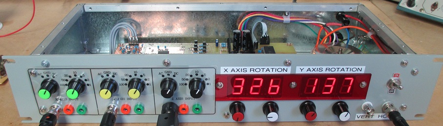
The digital heart of the system is microcontroller U9. U9 runs off a 5V digital supply rail and logic level shifting to communicate with the digital potentiometers, from 0-5V to +/-2.5V is performed by transistor switches Q7 through Q12. Transistor switches Q13 through Q16 provide logic level shifting to potentials appropiate for the gates of JFETs Q1 through Q6, of the switchable analogue inverting stages.

As already mentioned, the variable angles of rotation about both the x and y axes are set with "fine" and "coarse" control potentiometers. The positions of these mechanical potentiometers are continuously monitored by the internal ADC of uC U9, which programs the multiplication coefficents into the digital potentiometers as appropiate for the given angle(s) of rotation from values stored in a sine and cosine look-up table.

[1] Analog Computing at Ultra High Speed; An Experimental & Theoretical Study. Donald M. MacKay, Michael E. Fisher. John Wiley & Sons Inc. 1962