The Rössler attractor, originally discovered by German biochemist Otto Eberhard Rössler, is a system that exhibits continuous-time chaos and is described by three coupled,
ordinary differential equations. Rössler discovered a number of chaotic systems, including the first four-dimensional hyperchaotic attractor. However the system described here and thus dubbed the "Rössler attractor" is probably the most famous. The system is related to the
Lorenz system, but is simpler, generating a chaotic attractor having a single lobe rather than two. The equations are:
dx/dt = -y-z
dy/dt = x+ay
dz/dt = b+z(x-c)
The behaviour of the system is chaotic for certain value ranges of the three coefficients, a, b and c. The values originally studied by Otto Rössler were
a=0.2, b=0.2 and c=5.7. An excellent, and much more thorough introduction to the Rössler attractor, with references, is available at the Wikipedia page
here
While the Rössler attractor is readily simulated with iterative, discrete-type digital computation techniques on a modern desktop P.C., using software packages
such as MATLAB, or even in SPICE with a little more difficulty, it is also readily simulated with simple electronics hardware conforming to a much older concept;
that of continuous analog computation. A complete electrical analog of the Rössler attractor, as described by the three differential equations above, can be implemented
with an interconnection of just three distinct, basic and common circuit building blocks; namely the summing amplifier, the integrator and the analog multiplier.
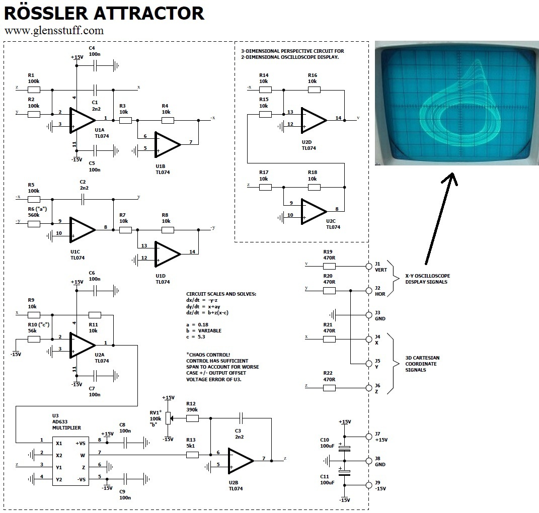
Here is my circuit that does just that:
In order to keep the computed and continuously-time variable
x,
y and
z state solutions within the linear operating range of the operational amplifiers
and the single analog multiplier chip running on +/-15V supply rails, a scaling (down) factor of 2:1 was used. Using standard value resistors, the
a and
c coefficient
values were set as close as practical to the values originally used by Otto, while the
b coefficient is made user-variable by means of potentiometer RV1. The oscilloscope pictures
below show, in successive stages, the effect of varying RV1, and thus the
b coefficient, over the full operating range.

A sufficiently high value of
b will cause oscillations to cease entirely, as depicted in the left-most image. This occurs with the wiper of RV1 positioned at the end of the most
negative potential (the
b coefficient is always a positive value, but U2B inverts the sign). As the wiper of RV1 is wound towards the positive, low-level oscillations eventually
begin, but they are simply periodic to start with. As
b is reduced in value further, the oscillations grow in amplitude and eventually become chaotic, and then increasingly more
so. Oscillations will eventually cease altogether once again, but this time at the other end of the range, if RV1 is advanced far enough. Excessively low, or negative values of
b
do not permit a solution nor sustained oscillation. Oscillations resume when RV1 is readjusted back within the permitted range.
The CRT displays pictured were produced with the oscilloscope in the X-Y mode of operation, with the corresponding Vertical and Horizontal signal inputs connected
to J1 and J2 as detailed in the schematic respectively. The Rössler Attractor is mapped in 3-dimensional space by the three coordinate values, x, y and z.
As the oscilloscope can only produce a display in the X-Y mode with two coordinate values at any one time, a transformation is required. This is achieved by U2C and U2D,
which generate the Vertical display signal for the oscilloscope by combining the x and z signals in such as way as to generate a 45-degree rotation to the perspective
of the (consequently) 3-dimensional projection along the horizontal axis of the display.
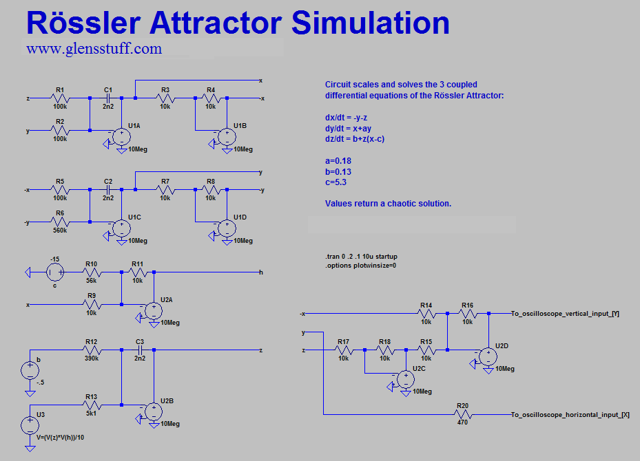
I produced a small PCB for the entire circuit as depicted schematically above; the Gerber files of which can be downloaded via the links at the top of this page, along with the LTspice simulation files. The operation of the circuit is simulated in SPICE with a simple transient analysis:

Well, that's it. In conclusion; a rather simple and unusual function generator that makes for a good, demonstrative introduction to analog computation and chaos theory - and a fun
weekend project as well.
